The Physics Behind The Phantom Issue 2 The Edge Phantom by Ken Freeman The Edge Phantom is designed to evaluate the imaging performance of Digital Radiography (DR) and Computed Radiography (CR) systems. The phantom and software as a system will measure the Modulation Transfer Function (MTF), the Noise Power Spectrum (NPS) and the Detector Quantum Efficiency (DQE). The methodology used to measure each of these characteristics will be discussed. In order to understand how the Edge Phantom measures and reports the MTF of the system it may be beneficial to review several mathematical concepts commonly employed in the evaluation of imaging systems in general. First is the Point Spread Function (PSF). This is the ultimate test of how well an imager reproduces the object being observed. The PSF simply says if an infinitely small point is imaged by the system how large would it appear in the resultant image. In other words, how much blurring will occur? Figure 1 shows a graphical representation of PFS. The vertical axis is image intensity and the horizontal axis is distance away from the point being imaged. Because the source is a point the result is three dimensional. The narrower the figure the less blurring there is and the better the spatial resolution of the imaging system. Figure 1 Point Spread Function The problem with using the PSF is the difficulty in obtaining a small enough point to image. To do so a hole would have to be drilled in some dense material small enough to allow only a few photons through and then there is the problem of having enough signal left to image. This method has been used, however, with a device called the pin-hole camera. One way to solve the signal problem is to use a slit instead of a small hole. This way more photons are transmitted and correspondingly more signal is generated. The image recorded when a line is used as an input to the imaging system is called the Line Spread Function (LSF). It is analyzed across the long axis of the image at any point. The crosssection image of the LSF is pictured in Figure 2.

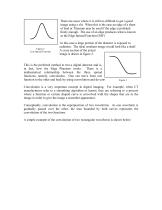
There are cases where it is still too difficult to get a good image using a slit. When this is the case an edge of a sheet of lead or Titanium may be used if the edge is polished finely enough. The use of an edge produces what is known as the Edge Spread Function (ESF) Figure 2 Line Spread Function In this case a large portion of the detector is exposed to radiation. The ideal resultant image would look like a shelf. A cross section of the actual image is drawn in figure 3. This is the preferred method to test a digital detector and is, in fact, how the Edge Phantom works. There is a mathematical...

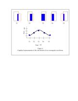
Time Figure 4 Graphical representation of the convolution of two rectangular waveforms

One can do the same mind experiment with the spread functions and see how by convolving the PSF with the line response of the system (essentially an impulse or very sharp rectangular signal) one arrives at the LSF and similarly LSF convolved with the step function yields the ESF. De-convolution allows you to do the process in reverse. A crude way to measure the spatial resolution of a system is to use a line-pair phantom. This phantom consists of a series of bars arranged such that the bars of a given width are separated by a space equal to the width of the bar. The bar widths range from large...

Modulation Transfer Function (Contrast) Spatial Frequency (LP/MM A more rigorous way of obtaining the MTF is to create the PSF of the system and apply a well known theorem known as the Fourier Transform. When this transform is applied to the PSF the result is the MTF. Now we have all the tools to understand how the Edge Phantom measures the spatial resolution response of a CR or DR system. First the ESF is obtained. The ESF is deconvolved into the PSF to which the Fourier Transform is applied resulting in the MTF curve for the system. The Edge Phantom Software also measures two other characteristics,...

computed for this image, a description of the frequency distribution of the noise is obtained. The NPS is simply the square of this data. Finally, with the data that we have already collected and a value that has usually already been stored in the imaging system we are ready to calculate the DQE of the detector. We do this by using the following relationship: DQE(f) = Where Φ is the quanta per mm2 received at the detector for the protocol being used and is a value that is generally stored in the memory of most digital imaging systems.